DC1 CFD techniques for IBRA-type discretizations:

Explore the use of IBRA-type discretizations in the context of CFD.

---

The Shifted Boundary Method in IGA

IGA has transformed computational mechanics by bridging the gap between Computer-Aided Design (CAD) and Computer-Aided Engineering (CAE). Originally introduced by Hughes et al. [1,2,3,4,5], IGA enables precise geometric representation and high continuity across element boundaries [6], making it an effective tool for simulating complex geometries [7,8,9]. The foundation of IGA lies in B-Spline and NURBS basis functions, which allow for smooth transitions and local refinement, enhancing the accuracy and robustness of simulations [10,11].
Despite its advantages, traditional boundary-fitted IGA methods face challenges with complex geometries, such as the need for watertight geometries and high computational costs in handling trimmed models [12,13]. Immersed boundary IGA methods, such as the Finite Cell Method (FCM) [14,15] and Isogeometric Boundary Representation Analysis (IBRA) [16,17,18,19,20], alleviate some of these challenges by using non-boundary-fitted discretizations. However, these approaches are often hindered by issues like the small cut-cell problem [21,22], which leads to poor computational performance and difficulty in solver convergence.

The SBM [23,24], initially developed within the FEM context, offers a promising solution to these challenges. SBM simplifies integration over complex geometries by shifting boundary conditions to a surrogate boundary and modifying boundary values using Taylor expansions. This approach avoids the small cut-cell problem, maintains optimal accuracy, and enables significant simplification in mesh generation and refinement. Previous applications of SBM in FEM have demonstrated its effectiveness in areas such as elasticity and incompressible fluid dynamics [25,26,27,28]. This study pioneers the integration of SBM with IGA, proposing an alternative to IBRA that eliminates the need for trimming techniques. By treating the boundary as unfitted, the proposed approach simplifies pre-processing and retains the accuracy and continuity advantages of IGA. The structure includes an introduction to the SBM framework, its application to the Poisson problem, and numerical validations.[31].

The Shifted Boundary Method (SBM) introduces key innovations.

• Surrogate boundary representation: the true boundary, denoted as Γ, is replaced by a surrogate boundary, which is constructed using the edges of a Cartesian background grid. This simplification avoids complications associated with small cut-cells in boundary-fitted methods (see Figure 1).
• Taylor expansion for boundary conditions: boundary conditions are imposed on the surrogate boundary using a Taylor expansion of arbitrary order mmm. This approach accurately approximates the conditions that would have been applied on the true boundary, preserving the desired level of accuracy.
• Weak imposition of boundary conditions: the shifted boundary operator is employed to weakly enforce Dirichlet and Neumann boundary conditions, ensuring numerical stability and compatibility with the unfitted nature of the method.

These features collectively enable SBM to achieve robust and accurate solutions without the computational overhead associated with traditional boundary-fitted approaches.

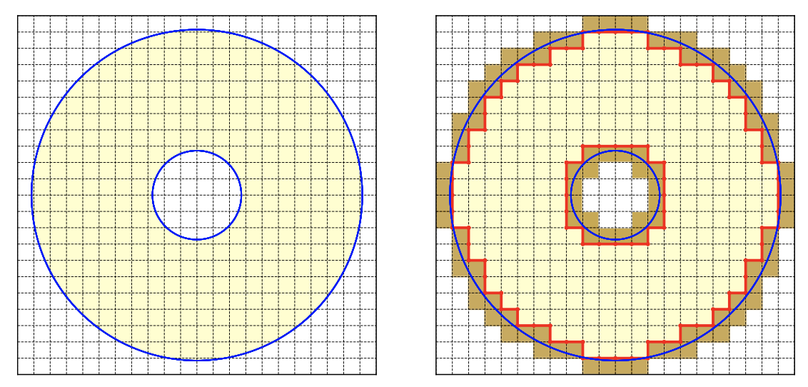
Figure 1: An example of a domain 𝛺 with a ring-like shape treated with the SBM in a Cartesian grid. Blue and red solid lines denote the true and surrogate boundaries respectively. The computational domain is shaded in light yellow, while brown denotes the intersected cells that are not part of the SBM computation.

The Taylor expansion plays a fundamental role in the SBM for accurately shifting boundary conditions from the true boundary to the surrogate boundary. This process involves performing an m-th order Taylor expansion of the variable of interest, u, at the surrogate boundary. Assuming u is sufficiently smooth within the strip between Γ and the surrogate​, the expansion incorporates directional derivatives along the vector d, capturing the influence of the distance between the true and surrogate boundaries.

The m-th order Taylor expansion includes a remainder term that becomes negligible as the distance ∥d∥ approaches zero. Dirichlet conditions defined on Γ are extended​ using the boundary shift operator, enabling the surrogate boundary to approximate the true boundary conditions. 

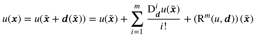
Neglecting the remainder term simplifies the boundary condition approximation to an m-th order shifted expression, which is subsequently enforced weakly in the SBM framework.

This approach ensures both computational efficiency and numerical accuracy while avoiding the complexities associated with direct boundary alignment [31].

Moreover, we have taken advantage of two ideas recently published:

1. Penalty-Free formulation: A penalty-free weak formulation [29] eliminates the need for penalty calibration, which is traditionally required for Nitsche’s method. The SBM variational form ensures numerical stability and accuracy without the overhead of parameter tuning.
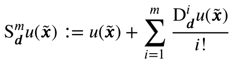
2. Optimal surrogate boundary selection: the surrogate boundary minimizes the distance function between the surrogate and true boundaries [30]. A parameter λ determines the inclusion of cut elements in the surrogate domain, with λ=0.5 found to be optimal for minimizing error.

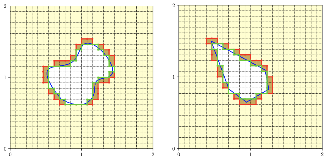
Figure 2: Selection of the surrogate boundary. Two-dimensional complex embedded holes treated using the SBM. The red solid line denotes the surrogate boundary corresponding to 𝜆 = 0 and the green one to 𝜆 = 0.5 (optimal surrogate boundary). 

In Figure 3 we report the convergence studies of the two cases in Figure 2 when applying only Dirichlet boundary conditions.

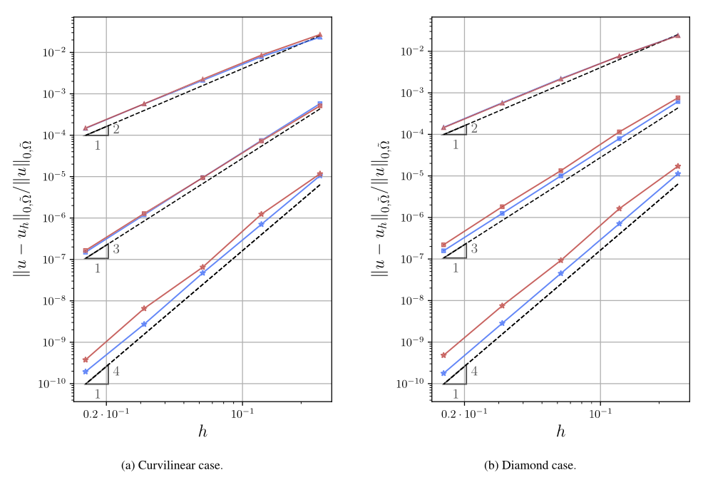
Figure 3: Selection of the surrogate boundary. Convergence study of two cases curvilinear and diamond of Figure 2  respectively, considering 𝜆 = 0 (red solid line) and 𝜆 = 0.5 (blue solid line). The order of the basis functions is indicated by the following symbols: triangles 𝑝 = 1, squares 𝑝 = 2, and stars 𝑝 = 3.

As previously mentioned, B-Spline basis functions are utilized to represent both the geometry and the solution fields. The implementation of the SBM avoids the use of trimmed knot spans, which are characteristic of the IBRA approach (refer to the left panel of Figure 4). The right panel of Figure 4 presents a comparison between the SBM and IBRA methodologies using linear, quadratic, and cubic B-Spline basis functions. The results demonstrate that both methods achieve very similar error norms and exhibit optimal convergence rates across all orders of the basis functions.

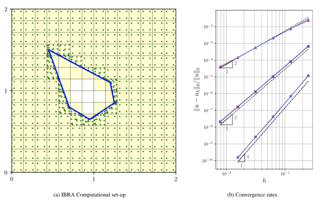
Figure 4: SBM vs IBRA. Left: the diamond shape applying the IBRA technique; the green dots denote the integration points, while the solid blue line highlights the true boundary. Right: the convergence analysis of the same case, using 𝑝 = 1 (triangular symbols), 𝑝 = 2 (square symbols), and 𝑝 = 3 (star symbols) and comparing the IBRA approach (red solid line) and the SBM (blue solid line) with the optimal surrogate boundary.

For more details and examples we refer to the paper “The Shifted Boundary Method in Isogeometric Analysis” [31], where the authors also analyze the case of Neumann boundary conditions.

SBM-IGA for Stokes fluids

This section explores the application of the SBM within the IGA framework to solve Stokes flow problems. The Stokes equations describe the behavior of viscous, incompressible fluids under low Reynolds number conditions, where inertial forces are negligible compared to viscous forces. These equations involve coupling between the velocity field and the pressure field, which introduces additional numerical complexity compared to the Poisson problem discussed in Section 1.

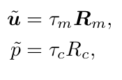
The Stokes problem consists of solving the following equations:

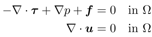
together with the boundary conditions. The weak form after integration by parts:

where v is the test function for the velocity vector field, and q is the test function for the pressure scalar field.

The Stokes problem is solved within a Variational Multi-Scale (VMS) [32-33] framework, which provides a stabilized formulation to handle the coupling of the velocity and pressure fields. In the VMS approach:

• The solution space is decomposed into resolved (coarse) and unresolved (fine) scales.
• Stabilization terms are introduced to account for the effects of unresolved scales on the resolved solution, enhancing numerical robustness and accuracy.

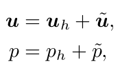
where

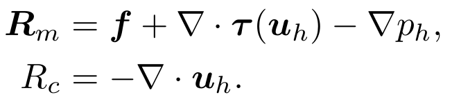
The VMS method, combined with B-Spline basis functions in the IGA framework, allows for arbitrary order discretizations of the velocity and pressure fields. Unlike the simpler Poisson problem, the Stokes equations involve higher-order terms that do not simplify directly, making the implementation of VMS more intricate. The weak formulation now is

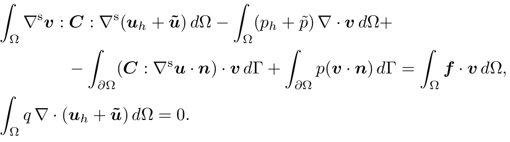
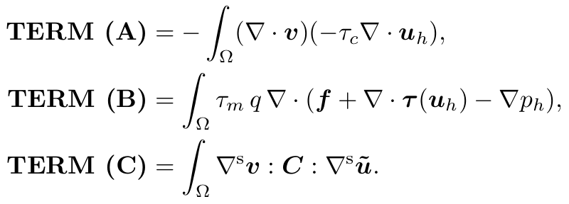
Therefore we have three additional terms with respect to a formulation without the sub-scale:

The implementation of the SBM for Stokes flow in IGA follows a similar strategy as in Section 1:

• B-Spline basis functions: The velocity and pressure fields are approximated using B-Splines of arbitrary order, ensuring smooth and accurate solutions.
• Shifted boundary conditions: Dirichlet and Neumann boundary conditions are imposed weakly on the surrogate boundary using Taylor expansions.
• Stabilization terms: VMS stabilization terms are added to the variational formulation to address numerical instabilities arising from the coupling between velocity and pressure fields.

The combination of SBM and VMS within the IGA framework enables the efficient and accurate solution of Stokes flow problems.

In addition to Stokes fluids, we introduced the use of  non-Newtonian fluids, specifically the Bingham fluid model. The Bingham constitutive law describes a material that behaves as a solid when the stress magnitude is below a certain yield stress and flows as a viscous fluid when the stress exceeds the yield stress. The stabilized formulation of the Bingham fluid incorporates an exponential factor that smooths the transition.

For small values of the regularization parameter, the behavior transitions smoothly between solid-like and fluid-like phases. Figure 5 shows the Stress vs Strain diagram.

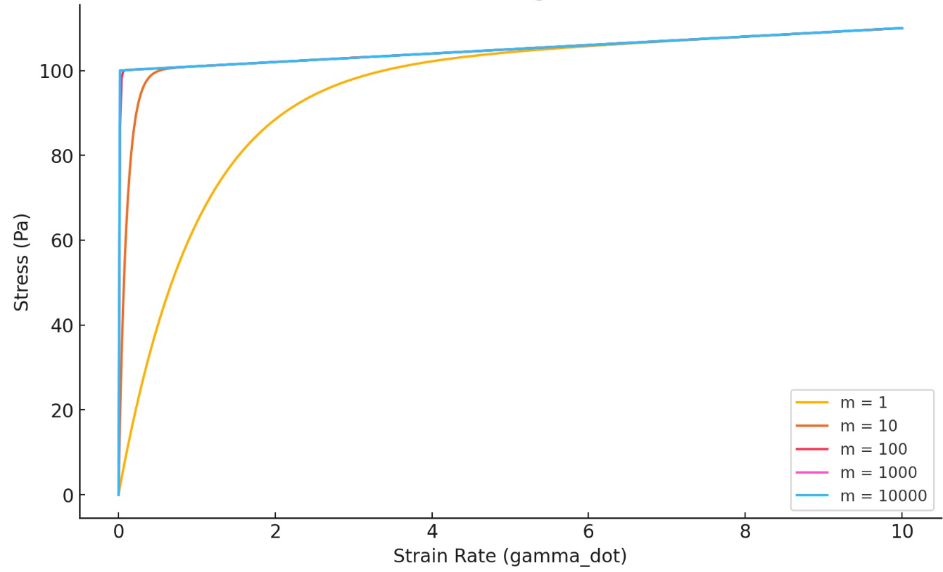
Figure 5: Stress vs. Strain Rate for the Bingham Model with Various Regularization Parameters (m). The graph illustrates the stress response of a Bingham fluid as a function of strain rate (gamma_dot​) for different values of the regularization parameter mmm.

We can show some preliminary results obtained with a manufactured solution for a Stokes fluid having a Bingham constitutive law. The manufactured solution is a smooth non-polynomial function in both the components of the velocity and in the pressure field. The convergence studies in the L2 norm of the error for velocity and pressure is shown in Figure 6 and Figure 7 (m = 10 and m = 300 respectively) for linear, quadratic, and cubic B-Splines basis functions.

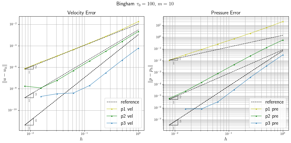
Figure 6: Convergence Study for Velocity and Pressure Errors with Yield Stress τ_0 = 100 and regularization parameter m=10. The figure shows the error convergence for the velocity (left) and pressure (right) fields as the mesh size h decreases. Results are presented for B-Spline basis functions of degree p=1 (blue), p=2 (red), and p=3 (cyan).

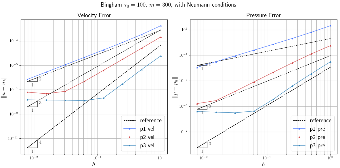
Figure 7: Convergence Study for Velocity and Pressure Errors with Yield Stress τ_0 = 100 and regularization parameter m=300. The figure shows the error convergence for the velocity (left) and pressure (right) fields as the mesh size h decreases. Results are presented for B-Spline basis functions of degree p=1 (blue), p=2 (red), and p=3 (cyan).

We observed that the exact solution must be smooth, including its derivatives, to achieve optimal convergence when using B-Splines. Unlike classical FEM, where the solution is typically continuous between elements, the IGA framework with B-Splines ensures continuity throughout the domain. If the solution exhibits discontinuities, particularly under nonlinear constitutive laws such as the Bingham model, the method fails to achieve the expected optimal convergence rates. Therefore, when applying IGA to problems with nonlinear laws, it is essential to ensure the smoothness of the solution to fully leverage the advantages of B-Splines.

We have also validated our code by testing it on the well-known lid-driven cavity problem, as illustrated in Figure 8, adapted from [34]. This benchmark problem is widely recognized in computational fluid dynamics as a standard test for assessing the accuracy and robustness of numerical methods applied to fluid flow simulations. The lid-driven cavity problem involves a square domain where the top boundary (lid) moves at a constant velocity, inducing circulation within the fluid. The remaining boundaries are stationary and impose no-slip conditions. This configuration creates a primary vortex at the center of the domain.

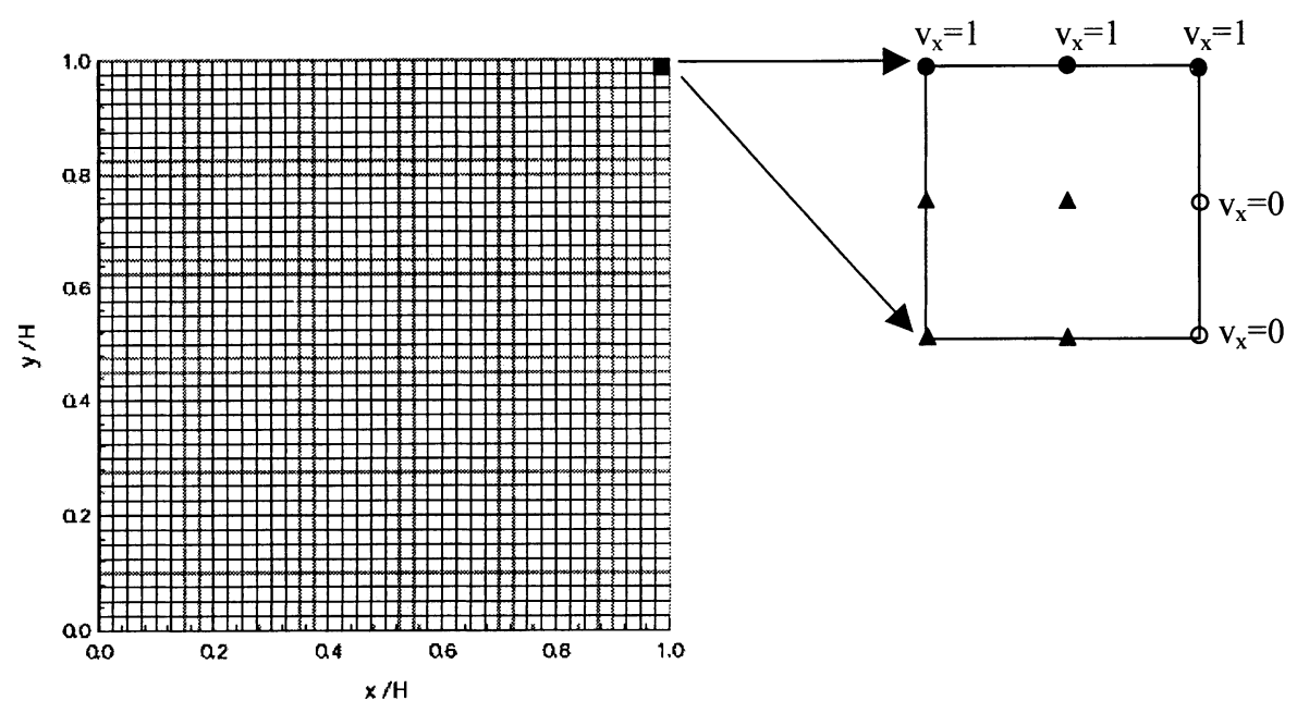
Figure 8: Cavity problem. The flow in a 2D cavity filled with a Bingham fluid. The problem is set up following Mitsoulis and Zisis [34]. Defining a square domain Ω = (0, H) × (0, H), we impose a horizontal velocity u_x = 1 m/s on the y = H.

Since no analytical solution is available for the lid-driven cavity problem, we have compared our results with the benchmark studies presented in [34] and [35]. This comparison focuses on two critical aspects of the flow behavior for different values of the yield stress: the extent of the yielded and unyielded regions within the domain, and the position of the eye of the main vortex that forms in the central-upper zone.
The yielded region, defined by areas where the fluid behaves as a viscous material, and the unyielded region, where the fluid behaves like a solid due to insufficient stress to induce flow, are key features of viscoplastic flows. Accurately capturing these regions provides insight into the robustness and precision of the numerical method (see Figure 9 and Figure 10). 

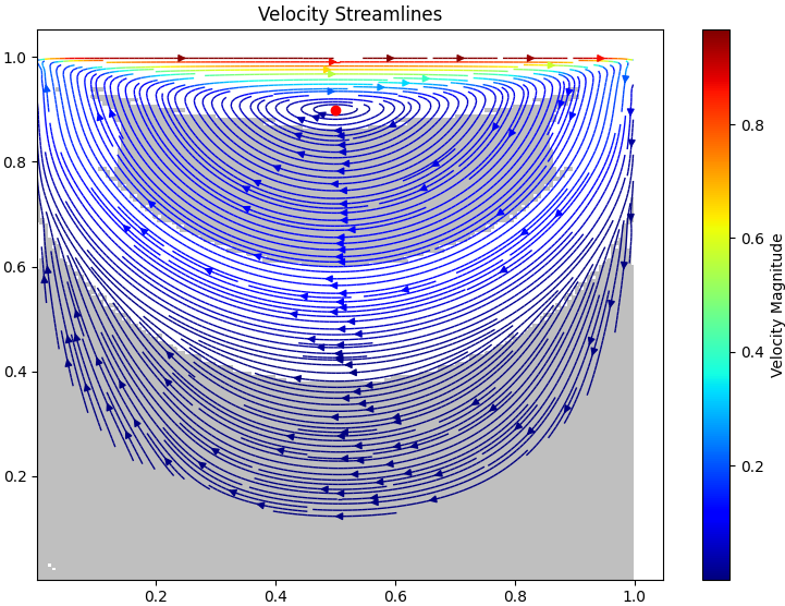
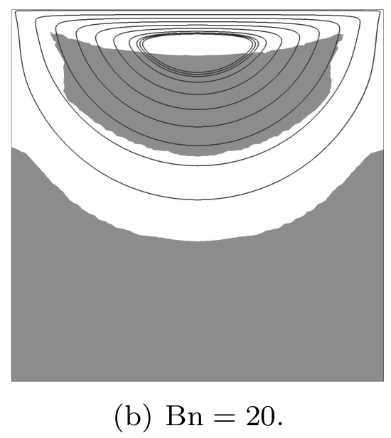
Figure 9: Yielded region. Comparison of the yielded region in the cavity flow problem. The Bingham number is equal to 20.0 and m = 300. Left: results with B-Splines with p=2 and 50×50 knot spans. Right: results in FEM from [35] using local refinement.

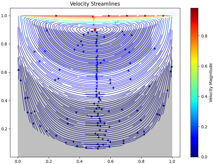
Figure 10: Yielded region. Comparison of the yielded region in the cavity flow problem. The Bingham number is equal to 20.0 and m = 300. Left: results with B-Splines with p=2 and 100×100 knot spans. Right: results in FEM from [35] using local refinement.

Additionally, the location of the vortex eye serves as an important indicator of the method’s ability to predict the flow dynamics accurately. The vortex position is influenced by both the yield stress and the imposed lid motion, making it a sensitive measure for evaluating the performance of our implementation (see Figure 11).

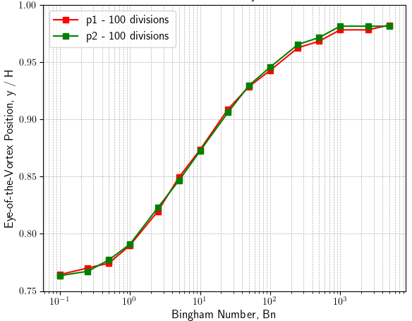
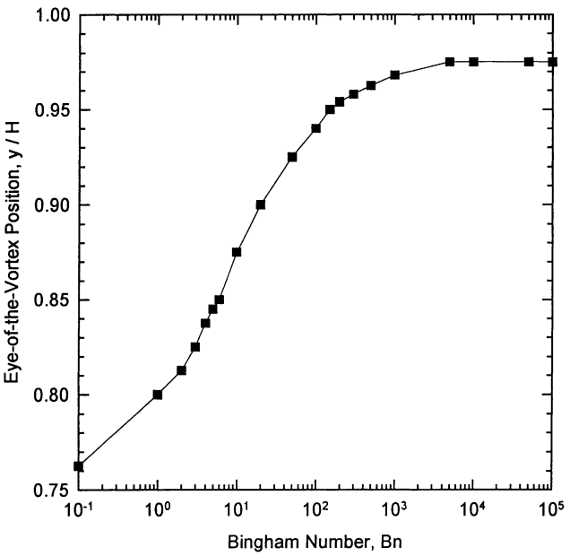
Figure 11: Eye vertex position. Comparison of the eye vertex y-coordinate in the cavity flow problem varying the Bingham number, m = 300. Left: results with B-Splines with p=1 & p=2. Right: results in FEM from [34] with 40×40 divisions.

Our results exhibit strong agreement with those in [34] and [35], confirming the capability of our Shifted Boundary Method (SBM) within the IsoGeometric Analysis (IGA) framework to handle complex boundary conditions and accurately simulate viscoplastic flow behavior in this classical benchmark problem.

REFERENCES

1. Thomas J.R. Hughes, John A. Cottrell, Yuri Bazilevs, Isogeometric analysis: CAD, finite elements, NURBS, exact geometry and mesh refinement, Comput. Methods Appl. Mech. Engrg. 194 (39) (2005) 4135–4195.
2. John A. Cottrell, Alessandro Reali, Yuri Bazilevs, Thomas J.R. Hughes, Isogeometric analysis of structural vibrations, Comput. Methods Appl. Mech. Engrg. 195 (41) (2006) 5257–5296.
3. Yuri Bazilevs, Lourenco Beirao da Veiga, John A. Cottrell, Thomas J.R. Hughes, Giancarlo Sangalli, Isogeometric analysis: Approximation, stability and error estimates for h-refined meshes, Math. Models Methods Appl. Sci. 16 (07) (2006) 1031–1090.
4. Yuri Bazilevs, Victor M. Calo, Yongjie Zhang, Thomas J.R. Hughes, Isogeometric fluid–structure interaction analysis with applications to arterial blood flow, Comput. Mech. 38 (4) (2006) 310–322.
5. Yongjie Zhang, Yuri Bazilevs, Samrat Goswami, Chandrajit L. Bajaj, Thomas J.R. Hughes, Patient-specific vascular NURBS modeling for isogeometric analysis of blood flow, Comput. Methods Appl. Mech. Engrg. 196 (29) (2007) 2943–2959.
6. John A. Cottrell, Thomas J.R. Hughes, Alessandro Reali, Studies of refinement and continuity in isogeometric structural analysis, Comput. Methods Appl. Mech. Engrg. 196 (41) (2007) 4160–4183.
7. Josef Kiendl, Kai-Uwe Bletzinger, Johannes Linhard, Roland Wüchner, Isogeometric shell analysis with Kirchhoff–Love elements, Comput. Methods Appl. Mech. Engrg. 198 (49) (2009) 3902–3914.
8. David J. Benson, Yuri Bazilevs, Ming-Chen Hsu, Thomas J.R. Hughes, Isogeometric shell analysis: The Reissner–Mindlin shell, Comput. Methods Appl. Mech. Engrg. 199 (5) (2010) 276–289, Computational Geometry and Analysis.
9. Kenji Takizawa, Yuri Bazilevs, Tayfun E. Tezduyar, Ming-Chen Hsu, Takuya Terahara, Computational cardiovascular medicine with isogeometric analysis, J. Adv. Eng. Comput. 6 (3) (2022) 167–199.
10. Massimo Carraturo, Carlotta Giannelli, Alessandro Reali, Rafael Vázquez, Suitably graded THB-spline refinement and coarsening: Towards an adaptive isogeometric analysis of additive manufacturing processes, Comput. Methods Appl. Mech. Engrg. 348 (2019) 660–679.
11.  Carlotta Giannelli, Bert Jüttler, Hendrik Speleers, THB-splines: The truncated basis for hierarchical splines, Comput. Aided Geom. Design 29 (7) (2012) 485–498, Geometric Modeling and Processing 2012.
12. Dominik Schillinger, Luca Dedè, Michael A. Scott, John A. Evans, Michael J. Borden, Ernst Rank, Thomas J.R. Hughes, An isogeometric design-through-analysis methodology based on adaptive hierarchical refinement of NURBS, immersed boundary methods, and T-spline CAD surfaces, Comput. Methods Appl. Mech. Engrg. 249–252 (2012) 116–150, Higher Order Finite Element and Isogeometric Methods.
13. Martin Ruess, Dominik Schillinger, Yuri Bazilevs, Vasco Varduhn, Ernst Rank, Weakly enforced essential boundary conditions for NURBS-embedded and trimmed NURBS geometries on the basis of the finite cell method, Internat. J. Numer. Methods Engrg. 95 (10) (2013) 811–846.
14. Jamshid Parvizian, Alexander Düster, Ernst Rank, Finite cell method: h-and p-extension for embedded domain problems in solid mechanics, Comput. Mech. 41 (1) (2007) 121–133.
15. Ernst Rank, Martin Ruess, Stefan Kollmannsberger, Dominik Schillinger, Alexander Düster, Geometric modeling, isogeometric analysis and the finite cell method, Comput. Methods Appl. Mech. Engrg. 249–252 (2012) 104–115.
16. Michael Breitenberger, Andreas Apostolatos, Philipp Bucher, Roland Wüchner, Kai-Uwe Bletzinger, Analysis in computer aided design: Nonlinear isogeometric B-Rep analysis of shell structures, Comput. Methods Appl. Mech. Engrg. 284 (2015) 401–457, Isogeometric Analysis Special Issue.
17. Tobias Teschemacher, Anna M. Bauer, Thomas Oberbichler, Micheal Breitenberger, Riccardo Rossi, Roland Wüchner, Kai-Uwe Bletzinger, Realization of CAD-integrated shell simulation based on isogeometric B-Rep analysis, Adv. Model. Simul. Eng. Sci. 5 (2018) 1–54.
18. Tobias Teschemacher, Anna M. Bauer, Ricky Aristio, Manuel Meßmer, Roland Wüchner, Kai-Uwe Bletzinger, Concepts of data collection for the CAD-integrated isogeometric analysis, Eng. Comput. 38 (6) (2022) 5675–5693.
19. Manuel Meßmer, Tobias Teschemacher, Lukas F. Leidinger, Roland Wüchner, Kai-Uwe Bletzinger, Efficient CAD-integrated isogeometric analysis of trimmed solids, Comput. Methods Appl. Mech. Engrg. 400 (2022) 115584.
20. Manuel Meßmer, Stefan Kollmannsberger, Roland Wüchner, Kai-Uwe Bletzinger, Robust numerical integration of embedded solids described in boundary representation, Comput. Methods Appl. Mech. Engrg. 419 (2024) 116670.
21. Erik Burman, Ghost penalty, C. R. Math. 348 (21–22) (2010) 1217–1220.
22. Santiago Badia, Eric Neiva, Francesc Verdugo, Linking ghost penalty and aggregated unfitted methods, Comput. Methods Appl. Mech. Engrg. 388 (2022) 114232.
23. Alex Main, Guglielmo Scovazzi, The shifted boundary method for embedded domain computations. Part I: Poisson and Stokes problems, J. Comput. Phys. 372 (2018) 972–995.
24. Alex Main, Guglielmo Scovazzi, The shifted boundary method for embedded domain computations. Part II: Linear advection–diffusion and incompressible Navier–Stokes equations, J. Comput. Phys. 372 (2018) 996–1026.
25. Nabil M. Atallah, Guglielmo Scovazzi, Nonlinear elasticity with the shifted boundary method, Comput. Methods Appl. Mech. Engrg. 426 (2024) 116988.

26. Efthymios N. Karatzas, Giovanni Stabile, Leo Nouveau, Guglielmo Scovazzi, Gianluigi Rozza, A reduced-order shifted boundary method for parametrized incompressible Navier–Stokes equations, Comput. Methods Appl. Mech. Engrg. 370 (2020) 113273.
27. Nabil M. Atallah, Claudio Canuto, Guglielmo Scovazzi, The second-generation shifted boundary method and its numerical analysis, Comput. Methods Appl. Mech. Engrg. 372 (2020) 113341.
28. Nabil M. Atallah, Claudio Canuto, Guglielmo Scovazzi, Analysis of the shifted boundary method for the Poisson problem in domains with corners, Math. Comp. 90 (331) (2021) 2041–2069.
29. Haydel Collins, Alexei Lozinski, Guglielmo Scovazzi, A penalty-free shifted boundary method of arbitrary order, Comput. Methods Appl. Mech. Engrg. 417 (2023) 116301, A Special Issue in Honor of the Lifetime Achievements of T. J. R. Hughes.
30. Cheng-Hau Yang, Kumar Saurabh, Guglielmo Scovazzi, Claudio Canuto, Adarsh Krishnamurthy, Baskar Ganapathysubramanian, Optimal surrogate boundary selection and scalability studies for the shifted boundary method on octree meshes, Comput. Methods Appl. Mech. Engrg. 419 (2024) 116686.
31. Antonelli, N., Aristio, R., Gorgi, A., Zorrilla, R., Rossi, R., Scovazzi, G., Wüchner, R. (2024). The Shifted Boundary Method in Isogeometric Analysis. Computer Methods in Applied Mechanics and Engineering, 430, 117228.
32. Codina, R., Badia, S., Baiges, J., & Principe, J. (2018). Variational multiscale methods in computational fluid dynamics. Encyclopedia of computational mechanics, 1-28.
33. Codina, R. (2000). Stabilization of incompressibility and convection through orthogonal sub-scales in finite element methods. Computer methods in applied mechanics and engineering, 190(13-14), 1579-1599.
34. Mitsoulis E, Zisis T. Flow of Bingham plastics in a lid-driven square cavity. Journal of Non-Newtonian Fluid Mechanics 2001; 101(1–3):173 – 180.
35. Cotela Dalmau, Jordi, Riccardo Rossi, and Antonia Larese De Tetto. “Simulation of two-and three-dimensional viscoplastic flows using adaptive mesh refinement.” International journal for numerical methods in engineering (2017).